
October 2021, Vol. 248, No. 10
Features
3-D Metal Loss Profiles from MFL Data
By Johannes Palmer and Andrey Danilov, ROSEN Technology and Research Center GmbH, Lingen, Germany
Magnetic flux leakage (MFL) data have high quality and coverage even under rough inline inspection (ILI) measurement conditions. The ILI vendor’s vast experience allows for heuristic MFL data evaluation, accepted by the pipeline industry based on hundreds of performance tests. Neural networks and artificial intelligence further improve the result probabilities. However, assumptions are never a definite calculation.
The conventional process allows for high performance but affects result repeatability and the value of run comparison. Moreover, it does not prevent outliers as the worst remaining defects. The responsible methodologically inherent MFL principal of ambiguity and the established simplification can be overcome: the groundbreaking Deep Field Analysis approach calculates 3-D profiles from MFL with high repeatability.
MFL Aspects
Reliable and accurate safe pressure prediction for corrosion features is of utmost importance for the safety of pipeline assets. Furthermore, only adequate repeatability permits corrosion growth assessments. However, MFL simplification tends to introduce conservatism and scattering. The established generalization may result in investigating metal loss features too early, with additional costs.
Nonetheless, even this conservatism, in some cases, results in erroneous data interpretation because of the inherent ambiguity associated with the nature of MFL data – the principle of going for the most probable shape does not guarantee picking the correct one.

The MFL signal is translated into an anomaly shape using existing knowledge from verifications, pull tests and synthetic data (Scheme 1). This process depends on assumptions and conditions supported by the knowledge from many thousands of experiences to optimally size a signal.
The use of artificial intelligence enhances the potential of the heuristic approach. Larger and more detailed data examples can now contribute. The discrimination is based and depends on the experience of the so-called “ground truth” stored in knowledge databases containing hundreds of thousands of anomalies, from pull tests and dig verifications to synthetic data. This not only improves the quality but also the level of detail of the solution, which then can comply with the new Pipeline Operators Forum (POF) requirements (POF 2020).
Individual pipelines and tool runs may introduce specific individual characteristics not fully covered by normalized ground truth data. Therefore, additional information from dig verifications, so called “calibration digs,” can help to adapt for bias effects and specific pipeline shape characteristics. This technique of “sizing model” adaptation is well established (Miller 2013).
Both artificial intelligence and calibration digs improve the heuristics (Scheme 1); unfortunately, they do not change the empiric nature. The stored knowledge and computing performance improve the detail, but the heuristic principle remains.
A typical example of such a MFL data translation is shown in Figure 1. Also, the inherent conservatism introduced by the box generalization is obvious. However, for a few decades now, this has made data analysis efforts manageable.
Breaking Boundaries
ILI metal loss sizing is one essential component of pipeline integrity management. Requirements regarding reliability, repeatability and level of detail of these data are increasing. Sizing discrepancies are often difficult to understand and manage. Overconservatism may cause high costs but still does not prevent interpretational outliers.
On the other hand, converting conventional MFL tool inspection data into metal loss geometry is not only extremely difficult, but the laws of physics do not allow for a unique solution. Established data interpretation is necessarily based on assumptions and simplification. However, a repeated check of the deviation between the synthetic magnetic field of such an assumption and the real MFL measurement is possible and suggests repeated refinement until the deviation disappears. This innovative principle is outlined in Scheme 2.
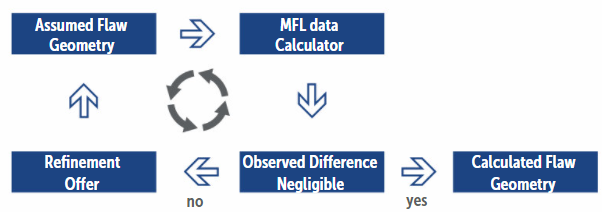
The MFL anomaly does not give the source geometry directly, but the other way around, directly deriving the MFL anomaly from a given source geometry is possible – the “MFL data calculator” in Scheme 2. Consequently, an iterative inversion process is possible, continually improving the assumption several thousand times until it fits the MFL ILI data. The successful fit is indicated by the difference approaching a benchmark stop criterion close to zero, which in Scheme 2 is called “negligible.” The resulting “calculated flaw geometry” is a calculated solution of the pipeline metal loss source geometry. This process is called “deep field analysis” (DFA) and used in the “virtual−dig up” (VDU) application.
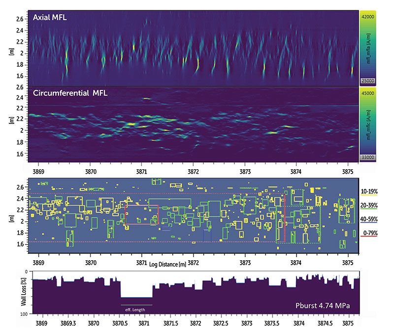
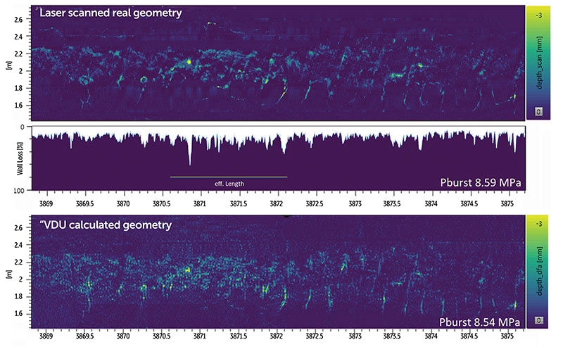
This process can run standalone or with combined MFL field directions – many thousands of times. Figure 2 shows the calculation results for the same location used in Figure 1, which is affected by complex external corrosion. In Figure 2, the results are compared with the laser scan. It is obvious how different the burst pressure calculations turn out. The VDU result (8.54 MPa) is nearly identical with the laser scan (8.59 MPa), while today’s simplification (4.74 MPa) is significantly overconservative.
MFL Ambiguity
A given flaw makes it possible to calculate the MFL magnetic field disturbance directly. This is called the “direct task,” while the “inverse” task, i.e., calculating the defect surface from a given magnetic field, is not possible. The academic jargon calls this expected MFL ILI industry requirement “incorrectly formulated” (Militzer 1984), because a scientist simply does not accept a question without a possible answer. Even metal loss flaws with non-exotic shapes but considerable depth differences (e.g., 29% vs. 52%) can cause the same magnetic field disturbance in the MFL signal (Danilov 2019).
All field directions (Militzer 1984) or different sensor-to-wall distances still cannot help. This MFL intrinsic principle, of course, also affects the process described earlier. Even a correctly calculated geometry solution for standalone MFL-A or MFL-C does not necessarily represent the correct geometry. Fortunately, the integration of MFL-A and MFL-C allows for uniqueness in this process (Danilov 2019). The integration of MFL-A and MFL-C requires vast efforts in the traditional empiric processes, which manual or parameter methods can only accomplish imperfectly.
The integration of these data sets with DFA, however, delivers much higher quality and even higher performance, because target model orientation and the prevention of wrong or implausible calculation paths actually accelerate the process. The result is not only the correct calculation but indeed the correct 3-D shape.
Blind Testing
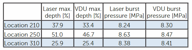
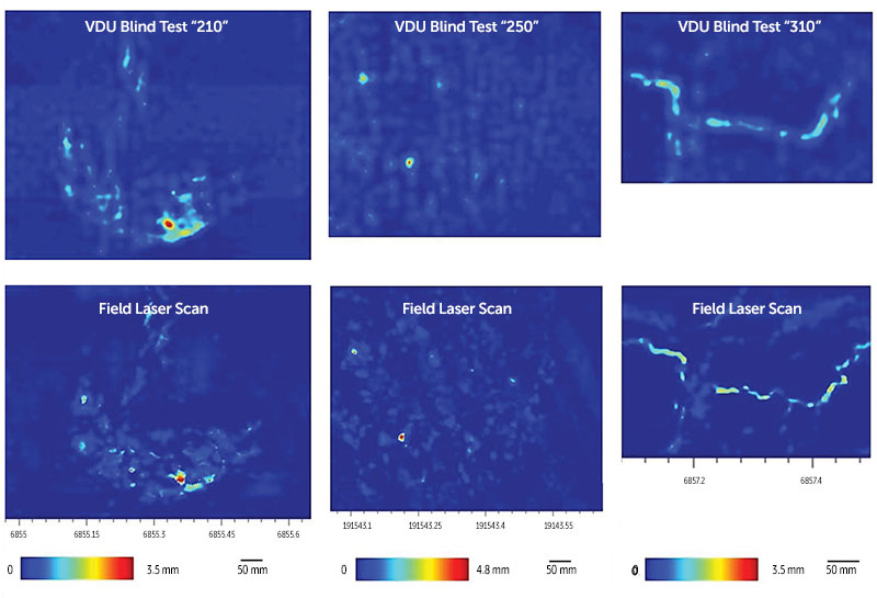
The results of a VDU blind test campaign (Palmer 2020) are shown in Figure 3 and Table 1. There are three locations of complex corrosion with general thinning (left), pitting (center) and slotting of varying directions (right). Table 1 lists the corresponding depth and burst pressure values, calculated according to ASME B31G, RSTRENG (ASME 2012).
A midterm perspective could be the stress calculation from the 3-D models via the von Mises equivalent stress, without a need for 2-D profile simplification. This forward calculation is available directly through the results data and requires only some refinement for adequate conservatism.
Summary
Converting conventional stand-alone MFL inspection data into metal loss geometry is impossible. Increasing knowledge and artificial intelligence further improve the result probability and principal potential of the heuristic approach. The pipeline industry accepts the empirical MFL data evaluation principle. Nevertheless, the best heuristic MFL assumption is not a definite calculation.
Artificial intelligence or calibration digs can help to improve, but do not change, this principle. Sizing model revisions do not principally change the ambiguity. Ambiguity means the wrong shape assumption may cause depth deviations significantly higher than specified. DFA and VDU solve ambiguity successfully by combining MFL-A and MFL-C.
Industry demands regarding repeatability, reduced conservatism and level of detail are on the rise. Three-dimensional metal loss geometry data are required. With the integration of MFL-A, MFL-C and inversion, MFL inversion is able to find mathematically correct 3D solutions. The described approach (DFA, VDU) can find the true and correct the 3-D solution. Laser-like metal loss profiles are achievable with MFL-ILI.
References
API Standard 1163 (2013), “In-Line Inspection Systems Qualification,” 2nd ed., Standard Publication, The American Petroleum Institute, Washington, DC.
ASME B31G (2012), “Manual for Determining the Remaining Strength [RSTRENG] of Corroded Pipelines,” Standard Publication, The American Society of Mechanical Engineers, New York.
Danilov, A., Palmer, J., Schartner, A., Tse, V. (2019), “Computing 3D Metal Loss from MFL ILI Data for Reliable Safe Pressure Prediction,” Proceedings of the Rio Pipeline Conference 2019, Rio de Janeiro, Brazil. “
Militzer, H., Weber, F. (1984), “Angewandte Geophysik – Band 1: Gravimetrie und Magnetik,“ Springer, Vienna, New York, Berlin.
Miller, S., Clouston, S. (2013), “Optimizing magnetic-flux leakage inspection sizing model performance using high-resolution nondestructive examination data,” in John Tiratsoo (ed.), Pipeline Pigging and Integrity Technology, Fourth Edition, Clarion, Houston, Texas.
Palmer, J., Danilov, A., Schartner, A., Tse, V., (2020), “Concerted, computing-intense novel MFL approach ensuring reliability and reducing the need for dig verification (IPC2020-9361),” Proceedings of the 13th International Pipeline Conference, Calgary, Alberta, Canada.
Pipeline Operators Forum (POF) (2016), “Specifications and requirements for intelligent pig inspection of pipelines,” Standard Publication, Version 2016, Amsterdam.
Pipeline Operators Forum (POF) (2020), “Specifications and requirements for Universal POF Template (UPT) data format for In-line inspection of pipelines” Standard Publication, Version 2020-11.

Comments