
September 2019, Vol. 246, No. 9
Features
Digital Alternative to In-Line Inspection
By Michael Smith, Konstantinos Pesinis and Matthew Capewell, ROSEN Group
There are two traditional schools of thought for monitoring internal corrosion in pipelines. One advocates the use of theoretical modeling techniques to predict the location, severity and behavior of corrosion; the other favors inline inspection (ILI) as a means to measure corrosion directly.
As the pipeline industry continues its digital transformation, however, we should acknowledge the prospect of a new solution for monitoring internal corrosion. ILI data continue to accumulate for pipelines all over the world, and for any given pipeline we can usually source data for similar pipelines that have been inspected in the past.
At the same time, the digital technologies to handle big data are becoming more sophisticated and efficient. This leads us naturally toward the concept of integrity analytics (IA) as an alternative to ILI. IA describes the process of predicting pipeline condition by learning from large amounts of historical data.
This article demonstrates the ability of IA to drastically improve predictions made using traditional modelling and provide a viable alternative to ILI.
Integrity analytics
The following analysis is based on data from a proprietary pipeline data warehouse. Data wrangling (collection, cleansing and structuring) and visualization were completed using the opensource programming languages python and r [1,2].

Figure 1 shows the distribution of internal feature count (per kilometer) for about 1,000 pipelines from around the world. Also shown is the distribution of feature depth (percentage of nominal wall thickness) for the about 7 million internal corrosion features reported within the pipelines. The data represent only a fraction of all ILI data in the world, but nevertheless provide a wealth of information.
First, it is clear that feature counts vary over several orders of magnitude, with counts below 10-2 km-1 at one extreme and over 10,000 km1 at the other. Nevertheless, the distribution has a heavy positive skew (implied by the approximate symmetry on a log10 scale) and a correspondingly low median in the order of 10 km1.
The implication is that pipelines with pervasive internal corrosion problems are very rare in the global context. In fact, fewer than 6% of the pipelines contain more than 80% of the internal corrosion. This inequality is reminiscent of trends in societal wealth, in particular, economist Vilfredo Pareto’s observation that 20% of people own 80% of the wealth [4].
Feature depths are also heavily positively skewed, with about 93% of all internal corrosion features reported with a wall loss between 10% and 20% (note that 10% wall loss is the ILI reporting threshold). Deep internal corrosion features are few and far between, with only 1 in 5,000 features reported at 50% wall loss or greater, and only 1 in 200,000 features reported at 80% or greater. Again, the implication is that severe internal corrosion is rare, present in only a small number of pipelines.
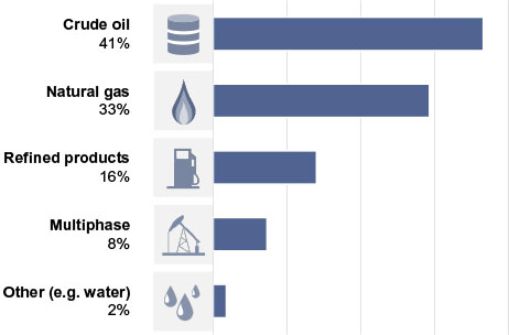
While we can already learn a great deal from the data, this basic summary clearly neglects the influence of key parameters – most notably the product composition. The database contains pipelines with a variety of transported products, as evidenced by Figure 2. It would be incorrect to assume that the general trends in Figure 1 hold true for all types of product, or indeed all process conditions or pipeline ages.
This highlights the challenge of learning from historical data; we must be very clear about the questions we ask, and we must carefully select the means by which we deliver answers. More specifically, IA can be broken down into three steps:
- Defining the problem – what exactly are we trying to learn?
- Selecting the data – which historical data are relevant?
- Learning from the data – what techniques should we use to learn from the data?
Each of these steps is explored in the following case study.
Defining the Problem
One of the most common tasks for operators of corroded pipelines is the estimation of corrosion growth rates (CGRs). CGRs support some of the most critical integrity management decisions that operators make, such as planning mitigation activities, identifying problem areas that require repair and estimating remnant life.
In the oil and gas industry, there are many different causes of internal corrosion, but carbon dioxide (CO2) corrosion is perhaps the most widespread. Predicting rates of CO2 corrosion is a notoriously difficult problem, with significant uncertainties due to variability between industry models [5] and high sensitivity to input data.
The prediction of CGRs in a pipeline affected by CO2 corrosion is therefore selected as a suitable example problem to demonstrate IA. Using IA, we attempt to improve upon results from the wellestablished corrosion model NORSOK M-506 [6].
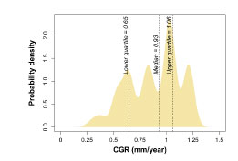
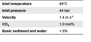
The target pipeline is a singlephase crude oil pipeline, with process conditions as shown towards the left of Figure 3. Following thermal and hydraulic modelling to extrapolate temperatures and pressures along the pipeline, the NORSOK M-506 model was used to make an initial estimate for the distribution of CGRs.
With a median value approaching 1 mm/year, the CGR estimates imply severe corrosion activity within the target pipeline. However, we know that the model results are highly uncertain and potentially unreliable.
The next step is therefore to source empirical data from the pipeline data warehouse and refine the CGR estimates.
Selecting the data
From the data warehouse, 14 similar crude oil pipelines were identified, each of which had been inspected twice using axial field magnetic flux leakage (MFL) technology. The ILI data contained about 83,000 internal corrosion features, attributable mainly to CO2 corrosion. For each feature, the local process data were also collected.
Given the size of the data set, assessing the similarity of the training pipelines with the target pipeline is not trivial. The tdistributed Stochastic Neighbor Embedding (tSNE) algorithm [7] was therefore used to support visualization of the data. tSNE is a dimensionality reduction algorithm that presents data points in a twodimensional space while preserving information about the local neighborhood of the points in the highdimensional space. Two points embedded in close proximity on a tSNE plot are also proximal in the highdimensional space.
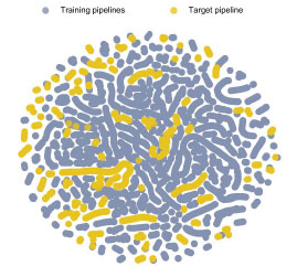
Figure 4 shows a tSNE plot representing the process conditions (temperature, pressure, CO2 content and fluid velocity) of the about 83,000 internal corrosion features from the training pipelines and about 6,000 features from the target pipeline.
The significant mixing of points for the training pipelines (blue) and the target pipeline (yellow) implies that they share similar process conditions. This in turn suggests that the training data will be suitable for learning.
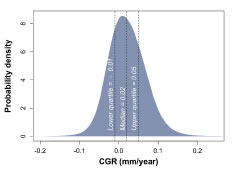
For each of the 14 training pipelines, CGRs were estimated using a “box matching” process [viii], a basic pattern recognition algorithm to compare features reported by the two MFL inspections. The resulting distribution of CGRs is shown in Figure 5.
While some aspects of the distribution are unrealistic (negative CGRs, for example, are physically impossible), the magnitude of the CGRs is more credible in comparison to the corrosion model.
Learning from Data
The final step is to update our prior beliefs from the corrosion model (Figure 3) in light of empirical evidence from the pipeline data warehouse (Figure 5). This is a typical Bayesian inference problem, which can be solved efficiently using a probabilistic graphical model known as a Bayesian network [9]. The solution was implemented in the commercial software Netica [10], and full details are given in [11].
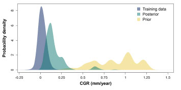
The final results of the IA process are shown in Figure 6, where the green (posterior) distribution is seen to be a combination of the yellow (prior) distribution and the blue (training data) distribution.
Interestingly, the posterior distribution has adopted the multimodal shape of the prior distribution (which reflects the variation in corrosion activity along the length of the pipeline), but with CGRs of a significantly reduced magnitude and scatter. Indeed, when compared to box matching CGRs for the target pipeline, the results of IA were found to improve the prediction accuracy by a factor of ~10 compared to corrosion modeling alone [11].
Conclusions
Integrity Analytics (IA) describes the process of learning from historical data in order to predict asset condition. This article demonstrated the potential of IA as an alternative to inline inspection (ILI) in pipelines.
In a case study for a crude oil pipeline, it was shown specifically that IA could improve internal corrosion growth rate (CGR) predictions relative to a wellestablished corrosion model. This was achieved using a Bayesian network trained on ILI and process data for 14 similar crude oil pipelines extracted from a global pipeline data warehouse.
IA improved the CGR estimates by an
order of magnitude relative to the corrosion model alone.
With additional development, it is expected that similar learning techniques could be used to predict the presence and behavior of external corrosion, cracking or bending strain in pipelines. P&GJ
References:
[1] W, McKinney. “Data Structures for Statistical Computing in Python,” Proceedings of the 9th Python in Science Conference, 51-56, 2010
[2] R Core Team. “R: A language and environment for statistical computing. R Foundation for Statistical Computing,” http://www.R-project.org, Vienna, Austria, 2013
[3] R. Palmer Jones, M. Smith, K. Pesinis, E. Santana and M. Capewell. “The good, the bad, and the ugly – categorizing pipelines using big data techniques,” Pipeline Pigging and Integrity Management (PPIM) Conference, Houston, TX, U.S.A., February 2019
[4] MEJ Newman. “Power laws, Pareto distributions and Zipf’s law,” Department of Physics and Center for the Study of Complex Systems, University of Michigan, Ann Arbor, MI, U.S.A.
[5] R. Nyborg, “Field Data Collection, Evaluation and Use for Corrosivity Prediction and Validation of Models – Part II: Evaluation of Field Data and Comparison of Prediction Models,” CORROSION NACE Expo 2006, Paper No. 06118, NACE International, Houston, TX, U.S.A., 2006
[6] NORSOK Standard M-506. “CO2 corrosion rate calculation model”, Rev. 2, June 2005
[7] L. van der Maaten and G. Hinton. “Visualizing High Dimensional Data Using t SNE,” Journal of Machine Learning Research, 9, pp. 2579-2605, 2008
[8] M. Smith, J. Martin, M. Peussner and K. Taylor. “Optimising corrosion growth predictions from in-line inspection data using Bayesian inference,” Technology for Future and Ageing Pipelines (TFAP) conference, Gent, Belgium, April 2018
[9] D. Heckerman. “A tutorial on learning with Bayesian networks,” Learning in Graphical Models, pp. 301-354, Springer, Dordrecht, 1998
[10] Norsys Software Corp. “Netica Application,” https://www.norsys.com/netica.html, January 2019
[11] M. Smith, K. Pesinis, L. Barton and I. Laing. “Intelligent Corrosion Prediction using Bayesian Networks,” NACE CORROSION Conference and Exposition 2019, Nashville, TN, U.S.A., March 2019

Comments