October 2019, Vol. 246, No. 10
Integrity Management
Improving Data Loss During In-Line Inspections
By Ahmad Al Saif, Engineer, Saudi Aramco, Pipelines Department
Using ILI technology to inspect hydrocarbon pipelines to revalidate the integrity of pipelines has been a common practice for many years.
Although there are other inspection methods, such as direct assessment or hydrostatic testing, ILIs are the most popular worldwide due to number of factors, including practicality, cost-effectiveness and accuracy.
Pipelines need to be periodically inspected to detect and measure any potential threat that might affect their integrity. Integrity threats can be divided into three main categories: metal loss due to corrosion, cracks and geometry damages.
Cracks are usually associated with high-pressure fluids, and the associated failures are usually more severe than metal-loss corrosion failures. Geometry damages (dents, wrinkles, etc.) in the pipelines are usually caused by excessive external stress on the pipelines. Each one of these threats require specific ILI technology to be detected and sized.
Metal loss corrosion is the main driver of pipeline deterioration and can lead to failures. In this article, only metal loss corrosion will be discussed.
The magnetic flux leakage (MFL) tool is widely used to inspect metal loss corrosion in pipelines. Upon completion of the MFL run, it must be validated by the pipeline operator. API-1163 standard offers three levels of validation for ILI run [1].
However, MFL runs might experience mechanical damage or electronic malfunctions for different reasons. Causes may include upsets in the operating parameters of the pipeline, partial closure of mainline valves or unexpected sudden sensor loss. Accepting such runs requires additional engineering analysis that will be addressed in the second section.
Data Loss
Data loss can be caused by many things including, but not limited to: sensor malfunction, sensor lift off the pipe wall due to excessive debris or sensor damage due to mechanical pipeline damage involving valves, guide bars or dents. API-1163[1] and CEPA[2] have addressed this issue and drawn the general guidance to validate the run, but neither standard specifies solid criteria for rejecting the MFL run.
The ILI vendor, however, must provide a summary of the number of malfunctioned sensors and the new detection and sizing criteria compared with the original one.
On the other hand, the Pipeline Operators Forum (POF) added more rigorous conditions to validate the MFL run in the: Specifications and requirements for in-line inspection of pipelines (2016)[3]. These conditions are:
- Continuous loss of data less or equal to 0.5 % of pipeline length.
- Discontinuous loss of data less or equal to 3% of pipeline length.
- Continuous loss of data from less than four adjacent sensors or 25 mm in circumference (whichever is smallest).
To put these conditions in perspective, let’s set an example of 56-inch pipeline with a total length of 62 miles (100 km):
- The maximum continuous data loss shall not exceed 500 meters, but it was not specified that the distance was the traveled distance or the trajectory distance with the circumferential coverage.
- The maximum discontinuous data loss shall not exceed 1.8 miles (3 km). Again, it was not specified that the distance is the traveled or the trajectory.
These two conditions were meant to cover axial data loss. Therefore, the third condition was set to define the limit of the circumferential data loss.
Analysis Guidance
When an MFL run experiences data loss, the ILI vendor shall provide the travelled path for each affected sensor to the pipeline operator. This raw data will be analyzed independently and combined with the previous pipeline corrosion data (such as, previous ILI runs and field findings).
The purpose of this analysis is to confirm the total data loss to be examined throughout the pipeline. Upon receiving the data loss log file, the following formula can be applied to calculate the coverage of each sensor:
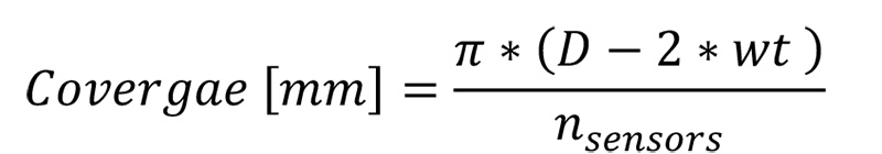
Where: [Cover gae [mm] = the total circumferential coverage per sensor
D = Pipeline diameter [mm]
wt = Nominal wall thickness [mm]
[nsensors] = Number of sensors per ring
Assuming each data point reports the center of the sensor, hence, the sensor’s coverage will be:
range [mm] = x [mm]± 0.5 * Covergae [mm]
Where: range = the range covered by one sensor from a given data point.
x = the reported distance of the defected sensor.
Now, one can specify the range at which the data was lost throughout the pipeline. An additional step maybe required to combine all adjacent defected sensors. With this data, the total axial and circumferential data loss can be calculated and represented in a similar format (Figure 1).
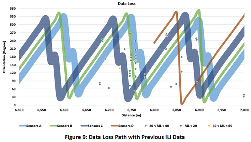
The presented figure would enable for more meaningful interpretation if it were aligned with the previous ILI corrosion data. Figure 8 aligned the two data sets and shows previous corrosion features with a metal loss depth of 40-60% were reported and locations correspond to the maximum data loss. For a similar case, the reliability of the new inspection is severely jeopardized due to the existence of deep corrosion features reported in the previous run.
Therefore, regardless of the overall quantity of data loss, pipeline operators shall take this section for more detailed analysis to confirm the reliability of this MFL run. For instance, a more detailed analysis would be to replace the distribution of the data loss (Figure 2) to the actual path of the defected sensors.
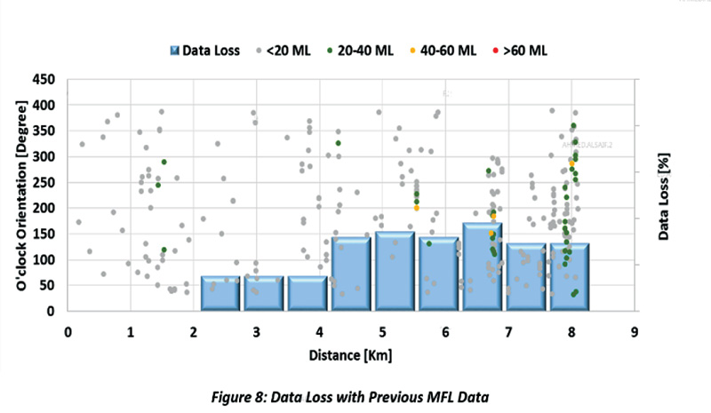
Figure 3 provides a snapshot of the combined path of the defected sensors and the previous ILI run results.
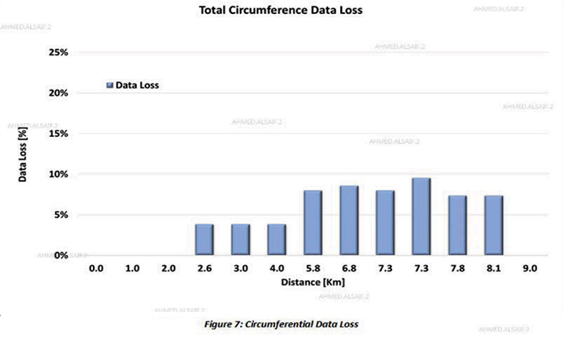
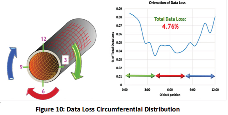
Clearly, there are corrosion features at the path of the defected sensors. A mathematical algorithm could be developed to find the distribution of the previous corrosion features that falls at the path of the defected sensors of the recent run. The last representation of the lost data is the distribution of the data loss along the circumference of the pipeline. Figure 4 illustrates that the total circumferential data loss is less than 5% and the least amount of data loss is at the bottom of the pipeline; which indicates that the MFL tool had a fair amount of rotation throughout the inspection run.
Therefore, the rotation of the tool can reduce the total missed corrosion features as the working sensors will have higher probability to catch general corrosion in the pipeline. It is worth mentioning that this analysis shall be aligned with the POF requirement that was previously mentioned.
Conclusion
This article introduced a new methodology to qualify an MFL run with partial data loss, which is consistent with API-113 and CEPA. The purpose of the methodology is to identify the criticality of the missed data based on a previous MFL run and to quantify the distribution of the missed data in both axial and circumferential range of the pipeline.
References:
In-line Inspection Systems Qualification, API-1163 STANDARD, 2nd edition, 2013
Metal Loss Inline Inspection Tool Validation Guidance Document, Canadian Energy Pipeline Association, 1st Edition, January 2016.
Specifications and requirements for in-line inspection of pipelines, Pipeline Operators Forum, 2016 edition.
Author: Ahmad Al Saif is a Saudi National engineer with a bachelor’s degree in mechanical engineering. He graduated from Pennsylvania State University in 2015.

Comments