August 2010 Vol. 237 No. 8
Features
Inertial ILI Results Guide Repair And Risk-Based Mitigation Decisions
An intelligent inline inspection run including XYZ mapping provides valuable input in various assessment methodologies and the automated integration of the accurate pipeline centerline with its physical properties into a central pipeline integrity management software allows for a cost-effective and time-saving enhancement of the accuracy and reliability of the assessments results.
This article looks at the software-aided process of this automated geographical pipeline centerline creation as the basis for a High Consequence Area analysis and how it is finally utilized to provide the necessary input on immediate defect criticality prioritization and a risk-based mitigation strategy.
Given that the task was one of developing a risk-based mitigation strategy for 7,000 km of liquid pipelines, buried onshore as well as offshore, the project was one that required a huge amount of input data to allow for reliable conclusions.
Looking to all the available sources, inline inspection data is primarily considered as the solution on the identification of the current situation on a particular piece of pipeline. But a combined XYZ mapping run not only provides valuable information on the geographical location of individual anomalies, it also provides information on prioritizing those by their immediate potential environmental impact as well as giving the most necessary input on a future consequence assessment: the actual detailed pipeline route and its interaction with nature and human settlements.
For the project under consideration here, API 1160 is the identified and named code to guide the operator on pipeline integrity matters. Among the immediate defect assessment reference was made to the code to tackle with that data also the following matters:
- Defect Assessment: “Anomalies located in or near casings, near foreign pipeline crossings, areas with suspect cathodic protection, or high consequence areas should take precedence over other pipeline locations with similar indications.”
- Risk Assessment: “The consequence is estimated as a combination of variables in categories such as environmental receptors, population, business interruption, spill size, spill spread, product hazard.”
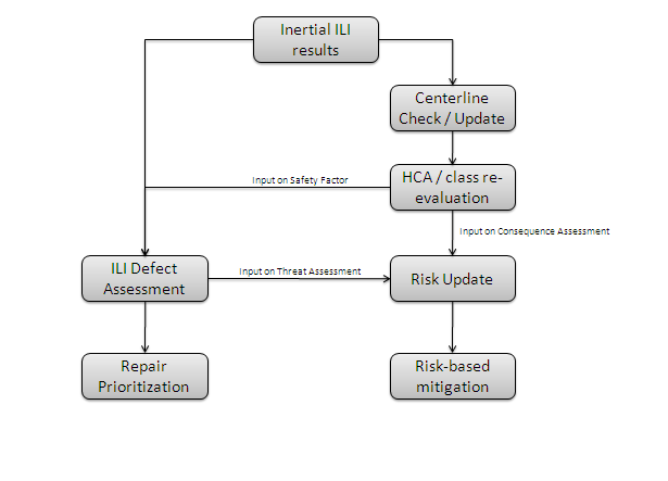
To support the responsible engineers in this process properly, a software solution was put in place that, among other capabilities, automatically integrates this data to update all related assessments performed in the various software modules provided. A generalized workflow is outlined in Figure 1.
XYZ Principles
XYZ Mapping has been developed for the identification of three-dimensional geographical pipeline coordinates by an inertial navigation unit. At the same time, the inner geometry of the pipeline is monitored simultaneously.
The survey results include information about the XYZ location of the pipeline, visualized by plan, elevation and distance views. Pipeline alignment, direction, horizontal and vertical bend orientations with respect to angle, radius, direction and location, are accurately measured, computed and reported. In addition, deformations such as dents, ovalities, wrinkles, etc. are also recorded. To get an indication on the setup of an XYZ Mapping Tool refer to Figure 2.

Figure 2: Setup of an XYZ Mapping Tool.
To achieve sufficient accuracy for absolute measurements, known reference points (in differential GPS ((DGPS)) position and GPS time) are required (Tie-Points). For this, above-ground bench markers are used, which are placed on known GPS reference points. The receiver of the marker is triggered by an on-board tool transmitter system. The GPS time at tool passage will be recorded by this system. Measuring the GPS position of the trap stations and line valves can generate additional reference points.

Figure 3: Accuracy of XYZ Mapping Tools.
The accuracy of XYZ Mapping tool results varies with the distances between Tie-Points and the velocity achieved during the tool run. The standard accuracy is defined with 3.3 feet (80% confidence). This accuracy is based on Tie-Points given every 6,500 feet and a tool velocity ? 2.6 ft/s. Furthermore, the GPS position must be surveyed with DGPS guaranteeing a horizontal accuracy of 10mm ±2ppm and a vertical accuracy of 20mm ±3ppm. The bench marker should be placed with an maximum offset of ±10cm to the GPS survey position. For accuracy details see Figure 3.
Centerline Creation
In the past, and still in various regions of the world, pipeline documentation is often based on one-dimensional formats that referenced different pieces of the pipeline route by stationing values. CAD drawings are in place, but often they visualized the two-dimensional impression of the pipeline based on local coordinate systems. Bringing the pipeline and its installations into a global spatial context allows analysis of the pipeline route and its installations together with various new aspects such as terrain, river networks or soil characteristics. Not only for the referred project, but also based on various other experiences, common data environments to create a digital pipeline centerline representation can be outlined as follows:
- CAD drawings containing geographical information;
- Shapefiles/Geodatabases;
- Technical documentation (XLS, PDF) containing facilities and pipe properties; and
- (Inertial) Inline inspection results.
Following the evaluation of the sources with highest accuracies, the immediate necessity is the creation of two combined consistent and accurate reference systems, the coordinate system in combination with the stationing system. These are commonly combined to the “XYZ + M” centerline environment used in the latest standardized data models.
The software-based process now uses the spatial alignment method “linear referencing” to combine the most accurate XYZ information – coming from inline inspections – with the stationing values mainly historically defined in the technical documentation. The pre-condition for this type of data alignment is the identification of identical reference objects in both datasets as the basis for an accurate calculation. In most cases, pipeline facilities like valves, taps, tees or makers are identified in the technical sheets as well as in the inline inspection data, so that the match-up can be performed. Finally, the overall mapping for the centerline and the physical parameters along the route looks like the following: (1) Centerline coordinates: ILI-XYZ mapping data, (2) Centerline stationing: Technical data sheets, (3) Pipeline physical properties: ILI-pipe tally data, and (4) Pipeline construction information: Technical data sheets.
The whole workflow of centerline creation is digitally implemented as an automated Extract-Transform-Load (ETL) process that directly writes the centerline representation into a common database system. In the case of this project the data model of choice is the Pipeline Open Data Standard (PODS) 4.0.
Following the alignment procedure, the sources are merged and the PODS database is automatically filled with the stationed centerline – the pipeline facilities as well as their properties and the respective geographical location of each object.
So when integrating an ILI run into the software, the operator can always decide whether this is solely for the purpose of evaluating the recorded defects or if he wants to make use of the extended geometrical and odometer reference as well to create or enhance the geographical location of his centerline.
High Consequence Areas
High Consequence Areas (HCA) are regions close to the pipeline centerline that could be affected in the event of a pipeline failure, either per leak or per rupture. Depending on the product and the pipeline transportation characteristics, different methods apply for the determination of regions that could be affected by a pipeline failure.
The case study this article builds on was performed on a liquid pipeline network situated outside the U.S., but in any case, U.S. regulations gave the basic definition for HCAs and the determination of those regions that could be influenced by pipeline failures. The U.S. regulations specify HCAs for liquid pipelines in CFR 49 § 195.450 and CFR 49 § 195.6. Parameters that need to be taken into account to determine which HCA could actually be influenced at pipeline rupture or leak scenarios are defined in U.S. CFR 49 § 195.452. For gas pipelines the model for determining HCAs considers – apart from transportation characteristics – mainly population data situated a certain distance around the pipeline centerline (U.S. CFR 49 § 192.903).
In the U.S. spatial datasets for navigable waterways, populated areas with different population densities and environmental sensitive areas are publicly available. Especially for U.S. pipeline operators, the National Pipeline Mapping System (NPMS) publishes regularly updated datasets storing HCA classes. This does obviously not reflect the situation found in other countries. The problems to be solved on the related project can be outlined as follows: (1) no homogeneous country-wide data infrastructure, (2) no consistent data related to HCA categories available, and (3) available data not up to date.
Consequentially, the encountered spatial data environment does not allow to directly implement HCA definition strictly following U.S. regulations. Based on the investigations made, a fitting definition for HCA determination is developed in accordance with the client and reliable sources are defined as follows: (1) census population units (where available), (2) river network, (3) road network, (4) natural parks, and (5) water intakes (where available).
Country-wide spatial terrain data and river flow directions cannot be considered for the determination of principally required transport zone analysis. Therefore, flow direction estimations of unplanned product release had to be replaced by conservative alternative models to determine HCAs that could be influenced by pipeline spills. In this case, pipeline centerlines were buffered for a distance that did not only account for possible product spill size amounts, but also applied a safety factor to consider possible spill scenarios.
Considering all available data and therefore the possible complexity level of calculations, the inertial mapping data including the identified installations are automatically facilitated in the software to provide the following: (1) centerline coordinates for geographical location of the pipeline and resulting calculation of direct intersections with HCAs, (2) elevation profile facilitated for spill size calculation and resulting conservative flow calculations for indirect impact zones, and (3) valve locations as additional input on spill calculations.
Figure 4: High Consequence Area evaluation.
As the result of the HCA calculation, the pipeline centerline is segmented for categories depending on the type of area they are intersecting as well as on the amount of areas they influence either directly or indirectly (Figure 4). These segments are then made available in the overall software context to eventually influence defect assessment and risk assessment calculations.
Immediate Defect Prioritization
To prioritize defects, the operator defines certain rules depending on isolated defect characteristics, e.g. “‘General’ corrosion features with peak depth greater than or equal to 60% wall loss” as well as on calculated properties considering additional pipe and environmental characteristics, such as “Features with an Estimated Repair Factor (ERF) greater than or equal to one inch. The ERF requires the Maximum Allowable Operating Pressure (MAOP), which itself depends on the class location. Checking the characteristics of this parameter, it should be reviewed occasionally, as population density changes and certain segments may no longer fall in the same category which was determined originally when constructing the pipeline. The defined procedure and software-based process takes into account these possible changes. The coordinate information from the mapping run is overlaid with the HCA evaluation and the revised MAOP is facilitated to calculate the ERF.
Considering a high amount of defects of the same criticality, i.e. with an identical prioritization based on the previously described rules, the software is able to consider directly the defects geographical location. This consequentially follows the guidance for prioritizing and scheduling anomalies based on API 1160: “Anomalies located in or near casings, near foreign pipeline crossings, areas with suspect cathodic protection, or high consequence areas should take precedence over other pipeline locations with similar indications.”
Next to the more comprehensive and accurate calculations on safety measures, the software is designed to support various filter mechanisms, considering the defect data in combination with the HCA outcomes. As API 1160 outlines, examples for such capabilities of a comprehensive data management software are as follows: (1) information and data can be sorted, filtered, or searched (e.g., list all corrosion defects with depths > 40% in HCAs), and (2) anomalies can be prioritized based on combined information (e.g., a corrosion spot in a specific location and in conjunction with a gouge).
Risk Assessment
The evaluation of risk caused by a specific segment of pipeline is the probability of it to fail because of a certain threat times the consequences in case of a failure. When deciding on the methodology to be used in the given project, the three commonly acknowledged types of assessments were up for debate: (1) qualitative risk assessments, (2) semi-quantitative risk assessments, and (3) quantitative risk assessments.
One crucial difference between those methods is the amount and detail of pipeline information needed to fulfill a certain assessment. When evaluating the different models against each other, an operator shall try to find the best balance between the complexity of the model, the available pipeline information and the effort that is to spent to populate the risk model with data. For the given project, a combination of a qualitative questionnaire approach and the input of “real” data was chosen. The model is thereby defined as semi-quantitative.
Even if the main goal of this chapter is to get a closer look on the consequence assessment, the threat assessment, which determines the probability of a pipeline failure, cannot be neglected. Differentiating in the broadest manner, the threat groups are differentiated by being time-dependent and time-independent: (1) time-dependent (external corrosion, internal corrosion, erosion, external stress corrosion, fatigue and ground movement, e.g. subsidence); (2) time-independent (third-party damage, sabotage, operating faults and ground movement, e.g. ground collapse).
Not to mention that ILI data specifically gives significant input on the presence of external and internal corrosion threats, the information gathered during those steps previously described helps extensively to get an indication on the impact on the different consequence categories to be considered: (1) direct input (impact of a failure on local population and consequence of a failure on local environment); (2) indirect input (legal impact, impact on company image, and economic costs to the company).
The type of pipeline failure – whether the failure is a leak or a full bore rupture – comes into play when conducting a consequence assessment. Among others, the consequence assessment is a function of the following parameters: (1) failure mode, (2) failure location, (3) fluid type, (4) pipeline pressure, and (5) pipeline diameter.
Establishing the consequence model for the different consequence categories, the factors of main importance are the HCAs, the estimated spill amount, as well as additional environmental factors that can be put into the model based on some qualitative input fields. It was also crucial to consider what information was actually available to feed the model.
The results derived from HCA analysis are incorporated for deriving the impact of a pipeline failure on the local population as well as for consequences of a failure on the local environment. In combination with the amount of spill following a leak or rupture and the additional identified questions, a simplified input model for these two categories is outlined in Table 1.
Table 1: Impact of pipeline failure on local population and local environment; outline of simplified model.
Impact On Local Population
* Input values derived from software internal calculations:
a) Number of affected high populated areas
b) Number of affected other populated areas
c) Segment spill volume (m3)
* Input parameters from consequence assessment questionnaire (identified sites):
a) Outside area or open structure
b) Building with 20+ persons for 50+ days/year
c) Major road
d) Railway
* Input parameters derived from product specification:
a) Toxicity factor
b) Flammability factor
c) Reactivity factor
Impact On Local Environment
* Input derived from software internal calculations:
a) Number of drinking water sources
b) Number of commercially navigable waterways
c) Number of unusual sensitive areas
d) Segment spill volume (m3)
* Input parameters from consequence assessment questionnaire:
a) Land quality
b) Accessibility and Clean-up time
The internal model itself is then combining the qualitative answers with the values coming from the direct data input. The consequence impact factors considering economic costs, legal costs and company image will not be explained further in this context as they are mainly based on consequence questionnaire input from the operator. The total consequence factor is the accumulation of the different impact factors mentioned in the Table.
Consequence = Economics + People + Environment + Legal (Eq 1)
Risk assessment results combine the probability of a pipeline failure derived from the threat assessment with the consequence of a pipeline failure derived from consequence assessments. A proper representation of those results is a matrix visualization where the borders for the X and Y axis are defined through corporate guidelines (Figure 5).
Figure 5: Risk Matrix visualization.
In the end, this visualization allows one to relatively rank each segment against each other on the probability of a failure and the consequence in case it happens. These results are valuable input for resulting verification and mitigation tasks.
Way Forward
The location information is already leveraged to a far extent and an immediate defect prioritization study has been completed where the result was a detailed short-term plan to mitigate these threats deployed. In addition to the assessments performed, further steps as a way forward can be explored from the results that the inspection run produced.
The initial review of the results of the internal inspection determined the characteristics (extent, location and dimensions) of the reported defects (corrosion, girth weld anomalies, dents etc.) and comments on the possible causes of the reported metal loss features such as field-joint coating breakdown. However, loading conditions (i.e., external axial or bending loads), could be selected and utilized to further assess the significance of the reported features. Therefore, the inline inspection data must be directly connected with e.g. information from SCADA systems to calculate loads along the route of the pipeline.
Considering the other identified defect types, an assessment of any reported dents applying strain-based assessment methods can also be explored along with reported manufacturing or construction type defects (reported mill faults and girth weld anomalies). Pressure-cycling data can be used to determine whether pressure cycle-induced fatigue crack growth is a threat to the integrity of the reported dents. This will determine if there is a risk of dent fatigue failure and if more detailed analysis is necessary.
Finally, looking not only at the immediate defect prioritization, but also at the future rehabilitation planning and inspection schedules, the assessment of defect growth mechanisms (e.g. corrosion) and the application of appropriate (agreed) rates of growth (for both internal and external corrosion as appropriate) will help extensively to estimate budgets on required upcoming integrity matters.
Conclusion
Inertial mapping data can be facilitated in various procedures defined in an integrity management program. Especially in those regions where the spatial component is not fully leveraged yet and the pipeline reference system is mainly distance-based, consideration to integrating an inertial mapping unit in the next inspection tool should be made. Various software programs as well as the standard industry data models that they support cope with most of the problems that arise from the huge amounts of data delivered throughout an inline inspection campaign.
This article describes how using current inline inspection technology aligned with available pipeline integrity software can accelerate the gathering of important accurate centerline data. This first step of gathering and ordering data was key in enabling a cost-effective pipeline integrity program along with prioritizing engineering decisions and accelerating the next phase of the integrity program. To a further extent, these additional methodologies and calculations can be automated, but in the end there should always be an engineering judgment when transforming calculated results into actions to be performed in the field.
Author
Markus Brors is executive general manager of ROSEN Integrity Solutions, a recently founded company within the ROSEN Group. For five years he has been involved in the product development of ROSEN’s client software products, as well as the project management of large pipeline integrity management software implementations and related services worldwide. He received his engineering degree in geo-informatics from the University of Applied Sciences in Oldenburg, Germany.
Acknowledgment
This article is on a presentation at the Pipeline Pigging & Integrity Conference in Houston in February 2010, organized by Clarion Technical Conferences and Tiratsoo Technical.
References
1. API 1160, Managing System Integrity for Hazardous Liquid Pipelines.
2. ASME B31.8S; Supplement to B31.8 on Managing System Integrity of Gas Pipelines.
3. United States Code of Federal regulations CFR 49 § 192 / 195.
4. The Pipeline Open Data Standard Association (www.PODS.org).
5. G. Weigold, C. Argent, J. Healy, I. Diggory, A Semi-Quantitative Pipeline Risk Assessment Tool for Piggable and Unpiggable Pipelines, IPC06-10280, Proceedings of IPC2006, Sep.25-29, 2006, Calgary, Alberta, Canada.

Comments