October 2011, Vol. 238 No. 10

Features

ILI Of New Rehabilitation System Uses Axial And Spiral Field MFL

A new technology for the external rehabilitation of pipelines known as Xhab® has been developed by Pipestream Inc. This technology involves wrapping multiple layers of ultra-high strength steel (UHSS) strip in a helical form continuously over an extended length of pipeline using a dedicated forming and wrapping machine.

The reinforcement afforded by the strip can be used to 1) repair a defective section of pipe (e.g., externally corroded or dented), adding strength to restore it to its original allowable operating conditions, or 2) reinforce an intact but de-rated section of pipeline (e.g., through a location class change) to maintain reduced hoop stress in the base pipe as required by codes and regulations, but allow reinstatement of the original MAOP by carrying the additional load in the strips..

One aspect of the technology to be addressed is how to confirm the long-term integrity of the repair and underlying pipe. The UHSS strip is a low-alloy carbon steel susceptible to corrosion if not properly protected. The system has three layers of protection, namely: 1) FBE coating on outer face of the outer strip, adhesive coverage of other strip faces; 2) overall protective coating over repair and adjacent pipe; and 3) electrical continuity between strip layers and pipe to provide cathodic protection via the pipeline’s existing system.

However, in the event that these layers of protection were to fail and the strip began to corrode, or if some other damage occurred to one or more of the strip layers at a particular location, it would be important to identify this and be able to reinforce or replace the pipe section before overall pipe failure occurs.

An inline inspection (ILI) trial has been performed on a test section of pipe containing an XHab repair with intentional defects in both the pipe wall and the repair strips. The trial was conducted by T.D. Williamson, Inc.(TDW) using an ILI tool containing both axial magnetic flux leakage (MFL) and patent-pending SpirALL™ magnetic flux leakage (SMFL) components. The trial has suggested that: 1) the location of the repair is easily identified using axial MFL; 2) large pipe wall defects can still be identified and measured beneath the repair using axial MFL, but there is considerable “noise” generated by the presence of the narrow strips and gaps in the repair; and 3) the noise is practically eliminated by the SMFL tool, which allows pipe wall defects and strip defects to be detected, subject to the defect being within the limits of the tool’s sizing specification.

Pull-through Trial
The identification of pipeline repair locations by the use of ILI tools has been an issue in the past where non-metallic composite wraps have been used since these are non-magnetic and therefore “invisible” to standard MFL tools. The XHab repair system, being a metallic composite, would not have the same problem as it is expected that the additional thickness of steel in the repair would give a clear indication of its location.

This trial was set up to test the “visibility” of the repair site to an MFL tool based on a test spool which would allow the following aspects to be assessed: 1) axial location of start and finish of repair; 2) resolution of pipe wall defect filled with epoxy filler material (both organic-filled and metal-filled epoxy); 3) resolution of individual UHSS strip layers in the repair; and 4) resolution of metal loss defects within strip layers (both above pipe wall defects and full pipe wall).

TDW was contracted to perform a pull-through trial at its Salt Lake City facility. Since strip failure is most likely from an axial defect across the width of a strip rather than helically along the length of the strip, TDW proposed the use of an SMFL tool in which the magnetization direction and sensor placement is arranged in a spiral, which provides better longitudinal defect detection.

Axial, Transverse And Spiral Fields
Axial MFL tools have been a mainstay of inspection for many decades. All MFL tools rely on the requirement of a defect to be large enough and oriented in such a way relative to the induced magnetic flux within the pipe wall to create a disturbance in the flux which can then be detected by the tool. Traditional MFL tools magnetize the pipe in the axial direction and are adept at detecting general metal loss and circumferential features, but do not reliably detect axially oriented features.

To address axially oriented features, many MFL vendors have developed transverse-flux inspection (TFI) tools which magnetize in the circumferential direction. TDW has developed a SpirALL MFL (SMFL) tool which is a TFI-type tool that magnetizes in an oblique, nearly 45- degree direction in order to detect axial features while still keeping tool length at a minimum.

The important point applicable to this study is that any feature that is circumferential will stand out in axial MFL data while axial features may not be detected. For the SMFL tool, the opposite is the case where circumferential features are not as detectable, but axial features will stand out. Figure 1 highlights this in a simplified manner with the arrows indicating lines of magnetic flux induced in the pipe wall by the respective tool type. Note that in the figure, circumferential MFL is shown 90 degrees to the pipe axis which is more representative of a typical TFI tool. While the SMFL tool’s flux is at an oblique angle approximately 45 degrees to pipe axis, the concept remains similar to TFI where axial anomalies are more effectively detected than with axial MFL.

Figure 1: Axial vs. circumferential flux direction and anomalies in pipe.

Fabrication Of Test Specimens
The test specimens were fabricated at Pipestream’s workshop facilities in Houston. The overall length of the pull-through spool is 24 feet, made up of three individual eight-foot sections in order to facilitate fabrication using Pipestream’s pipe prototyping machine. Each section had grooves machined into the ends to suit Victaulic connectors to allow the sections to be readily joined together.

The pull-through specimens were designed to include a range of defects, both in the base pipe and in the overwrapped strips. Three external defect depths were chosen (20%, 50%, 75% wall thickness) and spread over the spools. One defect of each depth was not wrapped in order to determine a comparison reading from the ILI tool. The rest of the defects were filled with an epoxy filler material as would be used in a field repair. The primary filler is an epoxy with an organic bulking material. However, three of the defects were filled with epoxy putty containing metallic bulking material to determine whether this would affect the ability of an MFL tool to detect the strips above.

The strip defects were cut-outs from each strip layer. Three layers were chosen to determine whether the MFL tool could discriminate between an inner layer, middle layer and outer layer. Three defect widths (measured circumferentially on the pipe) were chosen; 2 inches, 0.5 inches and narrow slit. Each defect length (axially along the pipe) was equal to one strip width (2.36 inches). The strip defects were placed both over full wall thickness pipe and above filled external defects. Three of each defect width and location was selected to determine repeatability of detection. Two “delaminated” areas were also built into each wrapped layer on one of the spools. This was achieved by not laying down adhesive over a quarter winding of the strip helix.

The carbon steel pipe selected was 16-inch NPS and 0.375-inch wall thickness. The diameter was chosen since 16-inch was the largest SMFL tool that TDW had readily available at the time of the test which met the lower end of the 16-30-inch range set for XHab machine No. 1. The range of the SMFL tool has since been revised. The wall thickness was recommended by TDW as being typical of the thickness of pipes of this diameter which they regularly inspect. In addition, the upper limit for magnetization of the SMFL tool is approximately 0.5-inches, so the pipe thickness plus strip thickness needed to be less than this for a reliable test. The pipe material was electric resistance-welded (ERW) rather than seamless to reduce variation in wall thickness around the circumference which could mask indications in the first layer of strip.

The strips were 2.36 inches x 0.04 inches ultra-high strength steel. The helical pitch was set at 2.48 inches, hence an average gap of 0.12 inches between adjacent windings of strip.

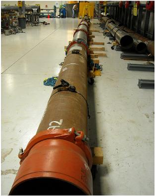
Figure 2 shows the construction process for the test spools in the following sequence: 1) filling the pipe wall defects with a stiff epoxy filler material prior to overwrapping; 2) wrapping the steel strip onto the pipe using a prototyping machine; 3) marking defect locations ready for cutting. Painter’s tape and careful placement of adhesive around the marked area allows the cut section of strip to be removed more easily; and 4) cutting defects into the strip, using a small electric cutting wheel. The figure shows a half-completed 2-inch cut. Photographs (e) and (f) show a typical completed cut, and overall completed spool. Note that “clock” markings were provided on each spool to ensure correct orientation during connection and to allow the results of the ILI run to be compared directly with the defect maps.

Figure 2: Construction of Test Spools.

The three test spools were arranged end to end and orientated circumferentially to ensure that the MFL traces would accurately reflect the defect maps. Lead-in and lead-out spools were connected to the overall pull-through length to ensure steady-state speed and magnetic flux was achieved within the test spools, as shown in Figure 3.

Figure 3: Pull-through Trial Set-Up (Including Lead-In and Lead-Out Sections).

Trial Results
MFL technology generally estimates metal loss defect depth in percent of nominal wall thickness, not in explicit depth such as inch or mm. This is mostly due to the way MFL signatures are created from pipeline metal loss features. MFL data interpretation is based on analyzing changes in magnetic fields detected by the tool in units of gauss and is not a direct measurement of wall loss. Defect dimensions including length, width, and depth are derived by analyzing magnetic field amplitudes compared to a background reading assumed to be nominal pipe wall thickness. Generally speaking, the larger the volume of metal loss relative to nominal pipe wall, the more effectively MFL will detect the anomaly.

For the pipe wall defects existing in the unrepaired pipe section shallow, medium, and deep wall loss defects appear in the MFL data. These relate to the defect depths of 20%, 50%, and 75% wall loss.

For the defects occurring in or under the repair wrap, it should be noted that nominal wall should actually be considered to be closer to 0.495 inches rather than 0.375 inches since three layers of repair wrap would add the equivalent of 0.12 inches to the base pipe wall thickness. In the case of the strip defects created by removing one layer of wrap, this would mean each strip defect would have an equivalent wall loss depth of only 8% wall (0.04 inches/0.495 inches). For a 50% pipe wall defect underneath the wrap, the addition of 0.12 inches of steel wrap to the nominal wall would give the defect an equivalent depth of 38%. Similarly, a 20% deep pipe wall defect under the repair would have an equivalent depth of 15% and a 75% anomaly would be 57%.

This effect is reflected in the depth sizing estimation in the actual MFL and SMFL data. While the defect length and width signatures remain constant in the raw data sets, the amplitudes of the anomalies are reduced when the defect is within the repair area that contains extra banding metal compared with the pipe outside the repair area. Since amplitudes are a main input into the depth sizing estimator for the MFL and SMFL tools, the anomalies under the repair would have a reduced depth estimation compared with when they are unrepaired.

The ILI tool was pulled through the spool section five times to test repeatability. It was orientated slightly differently for each pull to ensure that the circumferential variability in the magnetic field due to the spiral arrangement of the tool was considered. If a defect was picked up in the majority of these pulls, it was deemed to be “detected.”

The standard axial MFL tool was good at detecting the presence of the XHab repair i.e., the start and stop locations, and even the individual helical turns of the repair, but the “noise” due to the repair partially masked the pipe wall defects and completely masked the repair strip defects. Therefore, the Table 1 defect summary is based on detection with the SMFL tool only.

Table 1: Summary of Detection of Defects.

Key conclusions from the Table 1 results are as follows:

1) The pipe wall defects are detectable and measurable even under the repair;
2) The larger strip defects (0.5-inch width and above) are mostly detectable, both above good pipe and above pipe wall defects;
3) It is not possible to determine which repair layer a strip defect occurs in;
4) Even large strip defects can be masked by noise if they coincide with a sharp change in pipe wall thickness, such as at the edge of a pipe wall defect. This is the reason why one of the 2-inch defects was not detected;
5) A small strip defect may be detectable if it coincides with an area of reduced pipe wall thickness, such as in the middle of a pipe wall defect, and is on the inner layer of repair;
6) Voids or delamination due to lack of adhesive are not detectable using this inspection technology; and
7) No difference was reported between the results for the pipe wall defects with metal-bulked epoxy filler and organic-bulked epoxy filler i.e., the metal bulking in the epoxy is not sufficient to alter the magnetic flux at the defect.

MFL and SMFL traces for all three spools are shown in Figure 4. The MFL trace clearly shows the presence of the repairs, and the pipe wall defects are visible beneath the repair, but the “noise” created by the gaps between each helical winding masks any signal from defects in the strip layers. In the SMFL trace the strips are largely “invisible” and the extent of the repair is only evident as a slightly darker area associated with the increase in steel thickness in the repair region. The signals associated with strip defects can be seen in the SMFL trace for all three spools. However, these are particularly clear in Spool 2 where there are no pipe wall defects.

Figure 5 is a more detailed view of the SMFL trace for Spool 2 and includes an overlay of the strips and defect map. Note that the defects in strip layer 2 (red) are offset from layers 1 and 3 (green and yellow) due to the 50% overlap between adjacent layers.

Reviewing the specification of the combined MFL+SMFL tool, the defect depth required for a 90% probability of detection (PoD) ranges from 10% of wall thickness for general large defects, through 15% for axial grooving (mid-sized strip defects) to 25% for axial slotting (narrow strip defects). This approximately matches the detection rates in Table 1, where the only narrow strip defects that were found occurred over a substantial pipe wall defect where the overall steel thickness was lower.

It is important to note that the PoD values here would relate to apparent wall thickness of the base pipe plus steel repair strips, not just the base pipe thickness. Therefore, the number and thickness of repair strips relative to the base thickness is an important factor in how likely it is that a repair defect will be detected. If a larger number of thin strips is used rather than a smaller number of thicker strips, defects in an individual strip would not be as readily detectable.

(a) Axial MFL
(b) SMFL
Figure 4: Axial MFL and SMFL Traces for Full Test Length.

Figure 5: SMFL Trace for Spool 2 With Defect Map Overlaid.

However sophisticated ILI hardware and software may currently be, final interpretation of pipe defects from the data signatures is the responsibility of a trained human data analyst. One important fact that arose from the trial is that the MFL and SMFL traces for an XHab repair are not typical of those seen on a typical ILI run. However, even a minimally trained analyst would understand the axial MFL trace to be a man-made feature that would warrant further investigation with the pipeline operator as to its origin, particularly as it would also indicate a general increase in steel thickness beyond that of the base pipe.

In SMFL (or TFI), where the banding of the repair is not obvious, there is potential for a long XHab repair to be mistaken for a pipeline casing at a road crossing or similar. However, this should easily be confirmed by reference to pipeline alignment sheets or cross-reference to axial MFL data.

If XHab repairs are to be as widely used as hoped, it may be necessary to offer the major ILI operators the opportunity to perform pull-through tests as training runs for their analysts.

Conclusions
The following conclusions have been drawn from the pull-through trials performed by TDW’s MFL+SMFL tool on a section of pipe repaired by Pipestream’s XHab technology:

* Due to the signature that the repair wrap’s circumferentially oriented banding creates with axial MFL tools, defects in the pipe or in the repair itself may be masked and therefore undetectable by axial MFL tools. Transverse (or in this case SpirALL MFL) tools will have higher success at detecting anomalies under or in the repair.
* Depending on the nominal wall of the carrier pipe and how many layers of wrap are used for the repair, defects in a single layer of the repair itself may be difficult to detect. As the ratio of wrap thickness to overall thickness of steel from the pipe and the wrap combined decreases, detection will be reduced. MFL tool specifications should be cited to determine probability of detection for certain types of defects if their expected dimensions are known.
* MFL tools will generally not be able to determine if a defect is in the carrier pipe or the repair banding itself without prior knowledge such as detail on the anomaly that was originally repaired or a baseline inspection ran prior to the repair.
* MFL tools will not be able to differentiate which layer of the wrap may contain a defect.
* For any MFL tool, the geometry of a defect and total volume of metal loss which relates to depth, width, and length will dictate how effectively the defect will be detected. The same applies to defects in the repair wrap itself or any combination thereof. If defects such as active corrosion occur in the wrap itself, as more layers are corroded and lose metal or if the area of corrosion becomes larger, the more likely such an anomaly will be detected.
* Since small defects in the repair wrapping (or carrier pipe) may be more difficult to detect, it should be possible to run a baseline inspection using MFL shortly after a repair is made and compare it to subsequent inspections using the same tool technology. Changes from one inspection to the next would indicate issues with the repair or carrier pipe such as active corrosion, even if there is difficulty detecting or quantifying signatures under or within the repair. Some practical conclusions could be made with respect to the tool data to determine whether the pipe or banding is corroding. For example, if the original anomaly that was repaired was determined to not be internal corrosion, after the repair was made it could be assumed that the corrosion was stabilized. If subsequent inspections show increase of metal loss, it could be concluded that the issue is within the banding itself.
* While the machined pipe wall defects were created to represent corrosion, real corrosion anomalies are not so uniform in depth or dimension and may not be as large. In most cases, corrosion acts in more individual colonies. Even in areas of widespread general corrosion, there are usually localized areas where the anomalies become deeper, usually smaller in dimension than the width of the banding used in the repair. This may make it possible to find issues within the band itself more effectively.
* As the repair system starts to be used in the field, further work will need to be done to educate ILI contractors on the make-up of an XHab repair, and the typical signature of the repair itself and a defect within the repair.
* Continuity of tool usage from inspection to inspection will be important. The difference in signature between an SMFL tool and circumferential MFL tool may make it impossible to detect a repair defect if different tools are used for baseline and ongoing inspections.
* An alternative method is required to identify repair delamination (adhesive disbondment or missing adhesive). Internal inspection tools to detect pipeline coating disbondment are under development based on circumferential guided ultrasonic waves and the potential for this type of technology to be used is being investigated.

Acknowledgement
This article is based on a presentation at the 23rd PPIM Conference organized by Clarion Technical Conferences and held Feb. 16-17, 2011 in Houston.

Authors
David Miles, Ph.D., is technical director of Pipestream® Inc., Houston. He is a pipeline engineer with more than 13 years of experience in the oil and gas industry. He is responsible for providing technical direction for the developments of novel pipeline construction, repair and reinforcement methods. His duties include overseeing design methodologies, finite element analysis, full-scale testing and technology qualification programs.

Phil Tisovec is data analysis specialist for T.D. Williamson, Inc., in Salt Lake City, UT. He has a B.S. degree in engineering and more than 13 years of experience in oilfield and pipeline NDT environments. During his tenure with TDW, he has helped develop analysis processes, techniques, and software for TDW’s existing and emerging in-line inspection technologies with constant attention to customer needs.

Bibliography
Bond, T.J.M., Miles, D.J., Burke, R.N. and van Schalkwijk, R., 2010, “Testing and Analysis of Steel Strip Reinforcement for Pipeline External Rehabilitation”, IPC2010-31099, Proc. 8th International Pipeline Conference, Calgary, Alberta, Canada.

Simek, J., Ludlow, J. and Tisovec, P., 2010, “Oblique Field Magnetic Flux Leakage Inline Survey Tool: Implementation and Results”, IPC2010-31313, Proc. 8th International Pipeline Conference, Calgary, Alberta, Canada.

Venero, N.J., Burke, R.N. and Miles, D.J., 2010, “In-Field Application of Steel Strip Reinforcement for Pipeline External Rehabilitation”, IPC2010-31098, Proc. 8th International Pipeline Conference, Calgary, Alberta, Canada.