
September 2011, Vol. 238 No. 9
Features
One-Dimensional Modeling For Compressor Engine Controls
In modeling and control of power equipment, mathematical models are often used to develop robust control systems. The models are used both in the calculation of performance metrics and in determining control set-point parameters. These one-dimensional control functions require a method to determine an output value given some known input parameter. This article will describe various mathematical modeling methods that are used in compressor unit control systems as well as the advantages and disadvantages of each method.
One-dimensional mathematical models are used extensively in sophisticated modern control systems. Generically these models are:
y=f(x) (Eq. 1)
Where x is an independent variable and y is the desired output. A wide variety of functions are in control system implementations. Examples include:
* Establishing an ignition timing angle set-point as a function of engine speed,
* Predicting the specific power required for a reciprocating gas compressor as a function of compression ratio,
* Predicting the incremental fuel consumption on a two-shaft gas turbine as a function of off-optimum power turbine speed,
* Predicting the incremental fuel consumption on a reciprocating engine as a function of the engine torque,
* Establishing an air manifold pressure set-point as a function of the engine power,
* Modeling the operating limits of a synchronous generator (D curve), and
* The linearization of the signal output from a tank level gauge to the volume of fluid in the tank.
Three broad categories are used to represent these models. The first method is based on mathematic equations that represent the underlying physics. The second method employs curve fit equations such as polynomial, exponential, power, etc. The third method employs look-up tables. Variants to these methods will be discussed.
Physics-Based Models. Mathematic equation models based on physics are used where the underlying mathematics are well understood and the parameters in the equation are easily measured. Models of these types are often categorized as mechanistic models. As an example, the estimation of the inertia force from a reciprocating piston and connecting rod can be modeled as a function of crank angle using the following equation:
 (Eq. 2)
While this equation is relatively straightforward, it does have some limitations. For example, the equation includes a simplification using the series expansion approximation. In addition, the mass should include the mass of all reciprocating components (piston, rings, and if employed, piston rod and cross-head) and a portion (estimated at 2/3) of the mass of the connecting rod. Even though there are assumptions in using this equation, the equation is reasonably accurate.
Rotational velocity is easily measured and accurate in most control systems; all other parameters are constants with the exception of the instantaneous crank angle. In most control applications, it is not necessary to calculate the instantaneous force and, therefore, the instantaneous crank angle is not required. Instead, the peak forces are of interest and the angle range where the load is reversed on the connecting rod bearing (especially on a double-acting compressor piston), all are readily calculated using this formula provided the constants are known.
When using physics based values, one must be careful to make sure the parameters used in the equation do not result in numeric overflows. The most typical cause of numeric overflows is when a dynamic parameter (such as engine speed) is in the denominator and it approaches zero. Overflows can also occur when a parameter has an exponent such as the rotational velocity in the equation above. Careful data checking and memory sizing can avoid numeric overflow issues.
Curve Fit Equations. Curve fit equations are typically used where the underlying physics is generally known but too complicated to model in detail and the function is easily measured. These types of curves are generally considered to be empirical models. An example is determining the specific power required on a reciprocating compressor. To estimate the efficiency losses through the compressor cylinder (and therefore predict the power requirements), one must know the geometric details of the internal cylinder passages, compressor valves, and the geometry of the compressor cylinder. With this information, the gas flow velocities and static pressure losses can be predicted and the efficiency estimated. In contrast, an instrument can be used to measure the actual pressure in the compressor cylinder as a function of crank angle. With the basic cylinder geometry known (cylinder bore and stroke), the specific power can be measured.
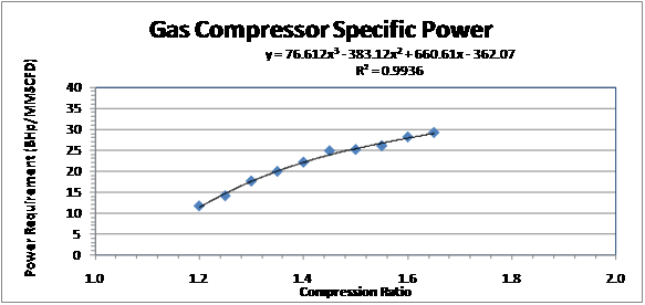
Most operators of large reciprocating compressors regularly use such instruments as part of their maintenance practice. The operator will gather operating information across a range of operating conditions that can be used to predict the required specific power requirements. Statistical data regressions are performed to fit the measured data to mathematical equations. An example is shown in Figure 1. The data is fitted to a third order polynomial using a least square method. A third order polynomial equation has the form:
 (Eq. 3)
The data fits reasonably well in this example with a correlation coefficient (R2) of 0.9936 (a value of 1.0000 is a perfect fit).
Figure 1: Third order polynomial fit of specific power requirements for a gas compressor.
Even with a good fit of the data, one has to be careful using curve fit equations in control systems. If the curve is not fit across the entire operating range, unpredicted results may be produced by the curve fitted equations. In Figure 2, the fitted curve is extended to compression ratios beyond the gathered dataset. From the graph we see significant deviations from the fitted curve (black line) to a curve characterized by the underlying physics. The error is especially large at compression ratios below 1.04 where the curve fit equation would predict the compressor is a power generator rather than a power consumer.

Figure 2: Same curve as Figure 1 with the curve extended to possible compression ratios.
When curve fitting data for control systems, it is always a good idea to include pseudo data in the dataset at the extreme ranges of expected operating conditions if measured values do not exist. This will help ensure that the fitted equation will provide reasonable values across the entire operating range. Figure 3 demonstrates adding reasonable pseudo points to the curve fit data set. Note that the predicted specific power is now much closer to the expected curve shape for operating conditions outside the test data set. In this case, adding the pseudo points did not significantly degrade the accuracy of the curve fit. The correlation coefficient is only slightly lower (0.9922) when compared to the curve fit without the pseudo points (0.9936).

Figure 3: Same curve as Figure 1 with pseudo points added.
Look-up Table Models. Look-up table models employ a series of discrete points. To determine the output of the function for all input values, an interpolation is performed using the points on the independent axis closest to the input for the independent variable. For example, using the five-point curve shown in Figure 4, the expected specific power requirement at a compression ratio of 1.65 yields an interpolated value of 30 BHp/MM/scfd. The look-up function is modeled reasonably well using just a few points.
Many different types of interpolation methods can be used to determine the expected output of the function between data points. The simplest and most common form is linear regression. However, linear regressions don’t always model a function well. Other interpolation methods include Newton series, cubic splines, Neville’s schema, and many others.

Figure 4: Same data as Figure 2 with a four-piece linear look-up.
Figure 5 shows an engine break specific fuel consumption curve as a function of engine speed. The four point linear look-up curve is reasonably accurate at engine speeds greater than 85% but is not generally accurate at speeds below that range. In this case, the third order polynomial fit curve is overall more accurate than the four point linear look-up curve. Note that as more points are added to the linear look-up curve, the accuracy using the look-up method is improved. This is achieved at a cost of additional computer memory and processor computational requirements.

Figure 5: Linear look-up table with insufficient number of points.
Zooming in to Figure 5 for engine speeds greater than 95%, as shown in Figure 6, the third order polynomial fit curve has some inaccuracies and falls sharply as speed increases. In this case, adding pseudo points to improve the accuracy at the higher speeds will degrade the accuracy of the curve at lower speeds.

Figure 6: Fuel curve detail with cubic spline.
An alternative to both the linear look-up and third order polynomial fit in this situation is to use a cubic spline look-up table. Cubic spline methods are a hybrid of polynomial curve fit and look-up tables. Each line segment between points has its own set of polynomial coefficients creating a piece-wise polynomial curve. An advantage of a cubic spline fit is it guarantees the curve will pass through each point in the table and the line will be a smooth curve as it passes through each point. Cubic splines can create wildly oscillating curves in some cases. The oscillation can be minimized in most cases by using polar splines or splines based on barycentric coordinate systems.
Other forms (other than polynomial) of piece-wise equations can be used as well. If piece-wise equations are used, care must be taken to ensure a contiguous curve exists at the transition point between curve segments.
When applied to a complex curve (a generator “D curve”), the largest absolute error for each method is shown in Table 1.
Table 1: Largest absolute error for each method.

A general comparison of the different modeling methods is shown in Table 2.
Table 2: A general comparison of the different modeling methods.

Modifying Data While Operating. For those times when control configuration data needs to be changed, it is beneficial to be able to do so while the equipment is operating. The ability to dynamically modify the control parameters while operating minimizes equipment outages and loss of production. Making changes while operating should only be performed by a trained professional using extreme caution.
Changes while operating should never be performed on control curves utilizing polynomial equations. To demonstrate why this is a problem, consider the modification of the gas compressor specific power curve shown in Figure 1 to the coefficients shown in Figure 3. As the A0 coefficient changes from -362.07 to -64.397, the curve jumps up to well over 250 BHp/MMscfd. Likewise, changes of the A1 and A2 coefficients also produce unrealistic control curves. It is not until all four coefficients are changed that the curve is restored to a realistic shape.

Figure 7: Changing polynomial coefficients.
Changing the parameters used in look-up tables can be performed while operating if the changes are made slowly and in small increments. Changing the control curve for tables using cubic splines should only be performed if the spline coefficients are dynamically recalculated when the tabular data changes. Like the look-up tables, changes should be made in small increments over a long period of time.
If there is any doubt as to the effect of changes to the control curves while the equipment is in operation, the changes should be performed when the equipment is not operating.
Conclusion
Mathematical models are regularly used in control systems for power equipment. Physics-based models are suitable where the underlying physics are well understood and the parameters can be accurately measured. When physics-based models are not suitable, there is a wide variety of interpolation models of which only a fraction have been presented here. For ease of use and accuracy, the linear look-up and spline methods are both accurate and reliable for use in control systems. Both methods facilitate changing the curve parameters while the equipment is operating if implemented carefully.
Author
Gary Choquette is a professional engineer with more than 25 years of experience in natural gas transportation. His expertise includes control equipment, hydraulic modeling, and optimization. He is a principal at Optimized Technical Solutions, Omaha, NE. Ph: 402-917-3395, www.optimizedtechnicalsolutions.com. Literature references for this article are available from the author.

Comments