
July 2010 Vol. 237 No. 7
Features
Clamp-on Ultrasonic Meters As Diagnostic Tools
Clamp-on ultrasonic flow meters are attractive to the gas industry because they are capable of providing portable, non-invasive gas flow measurement. This article describes the results of a Pipeline Research Council International (PRCI) funded project that addressed the ability of a clamp-on ultrasonic meter (CUSM) to measure distorted flow profiles.
The test approach was to traverse a single ultrasonic transducer pair around the perimeter of the pipe in sufficiently small increments to measure the flow field at a given pipe cross section independent of the amount of flow distortion present. Detailed profile measurements at the same locations were also made with a wedge probe. The intent of this testing was to determine the accuracy with which CUSM measurements, performed with sufficient spatial fidelity, can be used to provide a reference flow rate for in-situ meter proving.
The tests were conducted at Southwest Research Institute’s Metering Research Facility (MRF) in the High Pressure Loop (HPL) using transmission-grade natural gas (i.e., approximately 95% methane gas mixture) at nominal operating conditions of 800 psia and 70°F.
The 8-inch piping was arranged as shown in Figure 1 with a single 90-degree elbow upstream of a 139D (where “D” is the nominal pipe diameter) long, straight pipe run. The flow upstream of the elbow was conditioned using a Sprenkle flow conditioner followed by 43D of 8-inch pipe. Clamp-on meters were installed 12D and 126D downstream of the elbow. These locations allowed an existing velocity profile measurement spool to be installed such that the velocity probe could measure flow at the same axial location (downstream of the elbow) as the clamp-on meters.

Figure 1. Piping Configuration For The Meter Tests.
Data were collected simultaneously from the test meters and from the MRF HPL critical flow nozzle bank, which served as the flow rate reference. Five binary-weighted critical flow nozzles in the HPL nozzle bank were previously calibrated in-situ, at different line pressures, against the HPL weigh tank system (Park et al., 1995).
The volumetric flow rate reported by each ultrasonic meter was acquired through the use of the meter’s frequency output function. Each meter produced a pulse train where the pulse frequency was proportional to the flow rate computed by the meter. The pulses were counted using the MRF data acquisition system (DAS) and combined with pressure, temperature, and gas composition measurements to compute a mass flow rate that could be compared to the MRF reference flow rate. Although not discussed here, other meter-reported parameters, including speed of sound, path status, etc., were recorded using software from each meter manufacturer.
Pipe measurements were made at each of the meter installation locations. The outside diameter measurements were made using calipers, while the wall thickness measurements were made using an ultrasonic thickness gage. The diameters used to set up the meter electronics were based on the measurement of the pipe circumference (with a flexible tape measure) and the average measured wall thickness.
GE Sensing (GE) and Siemens each provided two clamp-on single path ultrasonic flow meters that were installed on existing MRF piping. The meters were set up in direct path mode, i.e., the transducers were installed on opposite sides of the pipe and the ultrasonic signal was not reflected off the pipe wall. The specific meters that were tested are shown in
Table 1. Each meter was tested at a single axial location, and the meters from a single manufacturer were tested simultaneously.
![]()
Table 1. GE and Siemens Meter Specifications.
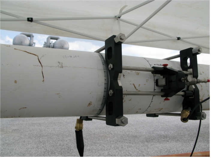
A representative from GE performed the setup and installation of the GE meters on the pipe. GE provided a fixture that was used to mount the transducers in direct mode, as shown in Figure 2. The standard installation of the GE transducers calls for damping material to be adhered to the pipe with windows cut in the material at the transducer location. However, the presence of the damping material would prevent the rotation of the transducers around the pipe. GE indicated that the damping could be left off for this test without affecting the results, since the pressure was high enough to allow an acceptable signal-to-noise ratio in the absence of the damping material. The rigid frame was clamped to the pipe and allowed the transducers to be rotated without risk of altering the axial separation between the transducers.
In preparation for the Siemens meter, the pipe was wrapped with a single layer of Grace Ice and Water Shield (used for acoustic damping) at the measurement locations. The damping material could be used with the Siemens meter, since the Siemens transducers clamp on top of the damping material as shown in Figure 3. SwRI staff received training from Siemens and performed the electronic meter configuration of both meters.
For both meter installations, flexible tape measures were adhered to the pipe to provide an axial reference position. The tape measures were marked such that the fixture could be rotated at 12-degree increments (a mark on the fixture was aligned with the marks on the tape measure). Each time the transducers were moved, the acoustic couplant material was cleaned from the transducers’ faces and a new coating of couplant was applied.

Figure 3. Siemens Meter Installation
Velocity profiles were determined by installing a pipe spool designed specifically for profile measurement and constructed such that the location of the profile measurement point was well defined. Four circumferential positions on the spool allowed an automated probe traversing system to be externally mounted without depressurizing the pipe or interrupting the flow. The pipe spool allowed the test probe to be traversed across the flow along a radial path.
Profiles were measured for bulk velocities equal to 55 ft/s and 33 ft/s at both the “disturbed” flow location (12D downstream of the elbow) and at the fully-developed profile location (126D downstream of the elbow). These were the same axial locations used for the clamp-on meter measurements.
For the profile traverses, dynamic pressure measurements were made at 45-degree increments using a 0.25-inch step size across the 7.981-inch inside diameter pipe. The pressure probe used for the measurements was a three-hole “W-probe” manufactured by United Sensor. The center hole of the “W-probe” arrangement allowed the determination of the total dynamic pressure, which was used to calculate the local velocity. The probe was rotated until the pressures at the two side ports were balanced. The probe rotation angle provided a measurement of the circumferential flow angle. Probe traverse, rotation, pressure measurement, and control of the system were performed through a combination of a stepper-motor-based motion control system and a PC-based data acquisition system.
Results
Each meter was tested over four flow rates with bulk velocities between 10 ft/s and 50 ft/s. At the highest velocity, a complete 360-degree rotation of the ultrasonic transducers was performed. At the lower velocities, the transducers were rotated only through 180 degrees. Tests were planned for velocities up to 65 ft/s, but initial tests indicated that the upstream meter was unable to function reliably at that velocity, presumably because of the profile distortion and turbulence present downstream from the elbow.
Once the tests were completed with both types of ultrasonic meters, the piping was rearranged to allow for velocity profile measurements to be performed at the same axial locations measured with the clamp-on meters. Velocity profile measurements were performed at two bulk velocities, Uavg = 33 ft/s and Uavg = 55 ft/s. These velocities bracketed the upper range of test flow rates used for the clamp-on meter tests.
The results provided in this section refer to the angular positions of the transducers and profile measurement device. This article uses the convention that zero degrees is a vertical path with the upstream transducer located at the top of the pipe. The indicated angle increased as the transducer was rotated in a clockwise fashion viewed opposite the flow direction (i.e., looking into the flow).
The plots that follow show results in terms of the meters’ measurement error relative to the HPL nozzle bank reference, i.e., Error = 100%*(Meter Flow – Nozzle Flow)/Nozzle Flow. The velocity profiles are provided in terms of a normalized velocity (u/Uavg) as a function of the normalized radial position. The normalized position is simply the ratio of distance from the wall to the measurement point divided by the pipe spool diameter.
Downstream Meter Measurements
Figure 4 shows the results for the Siemens meter when installed in the test position that was 126D downstream of the single elbow. The plot shows the meter error (relative to the MRF nozzle bank reference flow rate) as a function of the circumferential position of the transducers. These results were intended to provide an indication of the meters’ performance with a fully-developed flow. Results for four different test flow velocities are shown in the figure. The results indicated an error that varied with the circumferential mounting position of the transducers. This variation was initially thought to be related to the variation in the pipe wall thickness and diameter. However, the subsequent velocity profile measurements (e.g., Figure 5) suggest that the meter captured a slight asymmetry in the profile that existed even after 126D of profile development length.

Figure 4. Siemens Meter Results at the Downstream Test Location.
Integrating or averaging the results of the multiple circumferential measurements would not lead to a reduction in the measurement error, since the data had a bias error between 2% and 4%. Similar results were obtained using the GE meter. The bias in the error for both meters suggests a common measurement error source, such as the determination of the pipe diameter based on external measurements. However, this would require an approximate 0.040-inch (1-mm) error in the pipe diameter for each 1% error in flow. The likely error in diameter measurement was considerably less than the 0.12-inch (3 mm) error needed to account for the bias.
Figure 5 provides the results of the velocity profile measurements at the downstream test location for a velocity of Uavg = 55 ft/s. For a perfectly symmetric flow, the contour lines should be circular. However, the results indicate a slight asymmetry in the flow.

Figure 5. Contour Plot of Velocity Profiles (u/Uavg) Measured at the Downstream Test Location.
The profile measurements suggest that the variation in measurement error detected by the clamp-on meters was primarily driven by the profile asymmetry. This result suggests that mapping of the flow through multiple measurements with the clamp-on meters may be used to detect even subtle profile deviations. However, the overall measurement error would not necessarily improve through an integration of the results of multiple measurements of this type.
A contour plot of the velocity profile present 12D downstream of the single elbow is shown in Figure 6. The profile was significantly different from that obtained when the profile probe was located 126D downstream of the elbow. The upstream profiles suggest that the location of the profile disturbance was centered near the 50-degree angle. The location of the maximum deviation is somewhat surprising given previous measurements performed at the MRF (Grimley, 1998) where the “moon-shaped” area was centered on the 90-degree angle. Subtle differences in the piping between this work and the previous work may have created the change in the location of the maximum deviation. This result has implications for field testing: the velocity profile shape should not be assumed from the pipe geometry; it should be assessed in-situ, as described later in this article.

Figure 6. Contour Plot of Velocity Profiles (u/Uavg) Measured at the Upstream Test Location.
Figure 7 through Figure 10 show results when each meter was installed in the test position that was 12D downstream from the elbow. These results provided the meters’ responses to the disturbed flow profile of the type indicated in Figure 6. The cyclic nature of the measurement error was independent of the mean velocity, although slight differences in the position of the apparent maximum and minimum error points occurred for the lowest velocity test. Both meters indicated that the peak errors occurred near the 40-degree and 220-degree positions. Since measurements at these two positions occurred in opposite directions along the same diametral path, the error magnitude was expected to be the same, but opposite in sign. The extreme error values were within 1% to 2% of matching the expected behavior. The magnitude of the extreme errors varied slightly between the two meters; the GE meter measurement errors were 2% to 3% larger than the extreme errors indicated by the Siemens meter. The polar plots given in Figure 8 and Figure 10 provide another method of visualizing the disturbed flow behavior.

Figure 7. GE Meter Results at the Upstream Test Location.

Figure 8. Polar Plot of the Ratio of the Measured Velocity to the Average Velocity for the GE Meter when Installed at the Upstream Test Location (Uavg = 50 ft/s, 15 m/s).

Figure 9. Siemens Meter Results at the Upstream Test Location.

Figure 10. Polar Plot of the Ratio of the Measured Velocity to the Average Velocity for the Siemens Meter when Installed at the Upstream Test Location (Uavg = 50 ft/s, 15 m/s).
Application Of Results
For disturbed flows where there are asymmetries, there should be some sample location within the flow field that represents the average flow rate. In the absence of all other errors, a CUSM sampling at this location will provide the correct flow rate. Instead of attempting to integrate the profiles to determine the flow rate, another approach is to use a set of scoping measurements to determine the best location to make a measurement, or to determine which of the scoping measurements contains the best answer. The data suggest that if the CUSM is installed at a sufficient number of circumferential locations to determine the functional relationship between reported flow rate and position, the location with the minimum error (most correct flow rate) will be 90 degrees out of phase with the location of the minimum and maximum flow rates.
Using the approach just described, the meter output bulk velocity values were curve fit using an equation of the form:
Ufit = A + Bsin(?+?)
Where A, B and ? are constants and ? is the position of the transducers.
Table 2 summarizes the coefficients and the flow error computed based on the curve fit. The optimum measurement position is equal to the angle specified by ? (or 180 degrees away). The curve fit results indicate that the optimum location varied by approximately 10 degrees over the range of velocities tested. The magnitude of the estimated measurement error also varied with the bulk velocity and with the meter doing the measurement. A portion of the error can be attributed to slight changes in the velocity that occurred during the tests. For field applications where the flow rate is unlikely to remain constant for long periods of time, it may be necessary to install a second, fixed CUSM at a different location and use data from that meter to normalize the velocities recorded by the meter being rotated. The two meter configurations would allow the proper determination of the angular position for optimum measurement accuracy in the presence of the disturbed flow.

Table 2. Results of Curve Fitting Meter Output Data.
Conclusions
The results described here have shown that repeatedly mounting the CUSM transducers at different circumferential locations was an effective method of mapping the flow. The results for the well-developed flow testing demonstrated the ability of the CUSM to detect subtle profile deviations that were confirmed by an independent measurement of the velocity profile using a wedge-type pressure probe.
Data collected with both disturbed and well-developed flow conditions indicated that measurements at multiple circumferential positions cannot be used to remove bias errors. However, multiple measurements can be used to determine the best location to mount transducers to minimize the error due to flow distortions.
Additional testing with other types of flow disturbances, e.g., out-of-plane elbows, could be performed to assess if the methodology proposed here applies in general to other types of disturbed flows. This testing could be done initially at a calibration facility like the Southwest Research Institute Metering Research Facility, and then confirmed at a field location where custody transfer flow measurement is available. The advantage of testing at a field location would be that the flow variability would have to be accounted for and this would provide a more robust test of the suggested methodology.
Acknowledgements
This article is based on a paper prepared for the 2008 American Gas Association Operations Conference. This project was funded by the Pipeline Research Council International (PRCI). The support and efforts of the members of the PRCI Measurement Technical Committee are appreciated. The efforts of Mike Scelzo and Jed Matson of GE Sensing for arranging the use of the test meters is appreciated and Oleg Khrakovsky of GE Sensing performed the timely initial installation and meter setup. Ron McCarthy, Jim Doorhy, and Eli Spalten, of Siemens also provided test meters for the program and training to the SwRI staff.
The Author
Terrence A. Grimley is a Principal Engineer with the Southwest Research Institute, San Antonio, TX. He graduated from Purdue University with bachelor’s and master’s degrees in mechanical engineering and has worked at SwRI since 1986 on various flow related projects. Among these projects was the construction and commissioning of key components of the Metering Research Facility starting in 1991. He has worked with many different meter types and conducted research concerning ultrasonic flow meter performance and Coriolis flow measurement and contributed to the development of AGA Reports 9 and 11 covering those technologies. He is responsible for the flow measurement program at SwRI which includes operation of the Metering Research Facility and the Multiphase Flow Facility. Email: terry.grimley@swri.org.
Bibliography
Park, J. T., Behring II, K. A., and T. A. Grimley (Southwest Research Institute), Uncertainty Estimates for the Gravimetric Primary Flow Standards of the MRF, Third International Symposium on Fluid Flow Measurement, San Antonio, Texas, April 1995.
Grimley, T. A. (Southwest Research Institute), The Influence of Velocity Profile on Ultrasonic Flow Meter Performance, American Gas Association, Operations Conference Proceedings, May 1998.

Comments