
July 2010 Vol. 237 No. 7
Features
How Continuous Testing Further Reduces Gas USM Uncertainty
With the significant growth in the usage of ultrasonic meters, and industry’s drive for improvements, ongoing testing and development has resulted in enhanced performance of these meters. One such test was presented in 2009 at the CEESI USM Conference.
It involved testing two brands of 12-inch USMs with a series of elbows and tees upstream of the meter, and comparing the meter’s accuracy to a baseline consisting of straight upstream piping. A second test involving three elbows in and out of plane was also included in this test program. In addition to the upstream piping effects, the meter was not only tested in the upright (normal) position, but rotated 90° and rotated 180° (upside down) to see if the results were different.
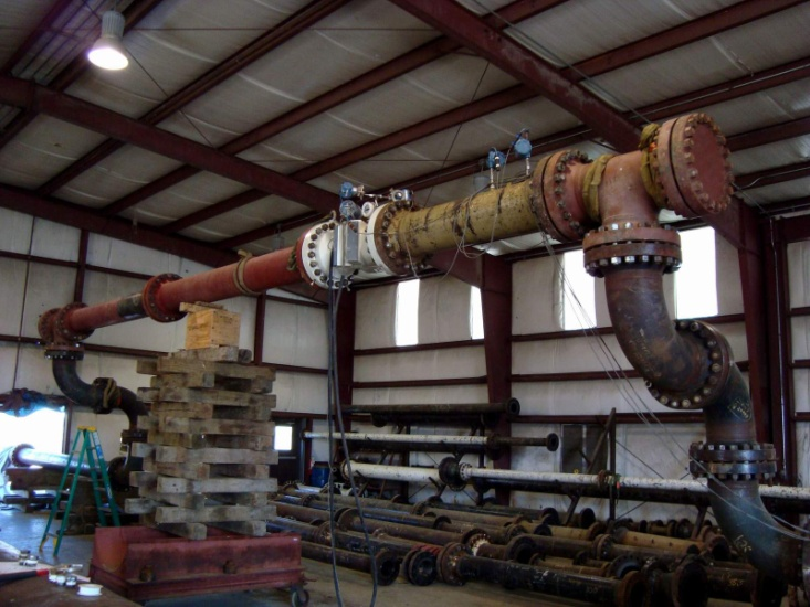
The meter run assembly consisted of 12-inch Schedule 40 pipe configured as follows: 10D + CPA + 10D + Meter + 5D. The meter was a FLOWSIC600 2plex 4+1 meter as shown in Figure 1. It consists of a conventional 4-path fiscal chordal meter and an additional independent single path meter incorporated into the same body. Each meter has its own independent electronics.

Figure 1: FLOWSIC600 2Plex 4+1 Meter design
For this article only the 4–path meter data is presented. The single path meter is typically used to identify added measurement uncertainty due to field conditions such as contamination. Since the testing was conducted at a calibration facility using clean, dry gas, the single-path data was not analyzed.
To establish a baseline, the meter run assembly was installed with straight piping (no elbows or tees) upstream of the assembly. The test data was collected at three flow rates (pipe velocities), approximately 20, 40 and 60 fps. After the baseline testing, the assembly was installed in a piping configuration consisting of three elbows and one tee upstream (Figure 2).One tee was used as this is typical of many customer installations. It permits internal inspection and cleaning of the meter run without removal from the pipeline. In addition to the meter being tested at the three flow rates, the rotational orientation of the meter was also added as a test variable. The entire meter package was rotated for these tests, not just the meter.
Since the data for the three elbows in and out of plane showed less than 0.05% shift, this presentation focuses on data from the more complex piping that included three elbows and one tee. The results showed a meter shift of +0.12% for the meter in its normal orientation, +0.13% with the meter rotated 90° and +0.22% with the meter package rotated 180° (upside down). See Figure 3.

Figure 3: Original CEESI test results

Figure 4: Meter Error – Before and After for Coefficient
Correction
Although the results were well within the AGA 9 required maximum of ±0.3% measurement uncertainty due to the installation effects, customer interest in the meter orientation effect led to further investigation at the manufacturer’s atmospheric test facility in Dresden, Germany. Although a different 12-inch meter was utilized, the upstream piping configuration and testing results were duplicated at atmospheric pressure.
This 4-path chordal meter employs the traditional Westinghouse® path configuration and weighting. It also incorporates a proprietary algorithm to compensate for distorted profiles that can occur due to field piping. The coefficients for the algorithm were developed in Europe using meter performance data with a variety of flow profiles including the OIML Installation Effects (R137-1).
The use of this algorithm helps reduce the effect of profile distortion that exists when no flow conditioner is used. Data on this testing was presented at the 2006 North Sea Flow Measurement Workshop (NSMFW) showing the benefits of this meter design [Ref 1]. A review of the CEESI test data resulted in identifying a minor error in the coefficients that resulted in slightly different results when the meter was mounted upside down. Although this difference was apparent in the 2006 NSFMW presentation, it was considered relatively insignificant.
This minor error was corrected and the testing was repeated at the Dresden atmospheric test facility. Figure 3 shows the plot of the original CEESI results (AvgVelGas = meter velocity). Figure 4 shows a chart of original results (dark red) and the same results with the new coefficient corrections applied (yellow). NOTE: Due to the open ended piping used at the atmospheric pressure lab, the upstream piping was rotated rather than the meter. As such TeeNormal = 0° meter rotation, TeeRotate = 90° meter rotation and TeeUpsideDown = meter upside down.
With the new coefficients, all shifts have been reduced ±0.03%, or less. This is well within the repeatability of the meter and calibration facility which is probably on the order of ±0.05%. To address any skepticism as to the validity of the testing and results based on atmospheric pressure testing, the high pressure tests at CEESI were repeated in September 2009 using the new coefficients. The same meter and piping used in the original CEESI testing was again used to repeat the tests, and thus validate the new coefficients derived from atmospheric testing. The results from tests with the three elbows and one tee are shown in Figure 5.

Figure 5: High pressure testing with new coefficients
As can be seen in Figure 5, the deviation from the baseline is virtually identical to the results predicted based on the atmospheric testing even though these tests were performed at pressures in excess of 1000 psig. This demonstrates that installation affects testing performed at atmospheric pressure can be replicated at higher pressures.
The next question that might be asked is: “What were the diagnostics telling us during the testing?” When dealing with field installation effects, the most important diagnostic is the velocity profile. Three aspects of the velocity profile, the velocity ratio, the profile factor and symmetry were obtained from the meter’s Maintenance Report files collected during the tests.
In order to answer the question of whether the new data collected in September 2009 truly represents the same profile (as seen in June 2009 from the original data), graphs from the September testing where the meter was rotated 180 degrees are presented in Figures 6 and 7. Only one data point is presented here in the interest of saving space, and the 180° rotation was chosen since it represented the largest shift from baseline.
These two graphs show the gas velocity profile is virtually identical to the June 2009 data. Some minor differences may have occurred since the meter piping, including the flow conditioner, had been disassembled between the June and September testing.

Figure 6: Comparative Path Velocity ratios for 180°
Rotation
Figure 7: Comparative Profile Factor & Symmetry
for 180° rotation
Some may contend that this data only applies to the 12-inch line size. To answer that concern, a second series of tests was conducted on a 6-inch meter in April 2010. The piping configuration was identical with three elbows and one tee upstream of the meter run assembly. Figure 8 shows the results of the baseline and upstream installation effects.

Figure 8: 6-inch Meter Testing Results – Three Elbows and One Tee (April 2010)
The results were similar to the 12-inch data, but with a slightly higher shift (less than 0.07%). This is probably due to the influence of the transducers since the same size of sensors are used in both the 6 and 12-inch meters.
As the meter size diminishes, port influences can have minor impacts in meter performance. However, with an average effect of 0.066%, most would feel this is within the repeatability of the system, and certainly well under the uncertainty of the calibration laboratory.
Conclusions
Today the importance of having accurate measurement has never been more important. The extensive use of USMs during the past several years has helped many companies continue to reduce their Lost and Unaccounted For (LUAF) gas. As technology continues to improve in all aspects of measurement, the highest uncertainty of any gas measurement device continues to be the primary element. Transmitters are regularly calibrated to accuracies of less than 0.1% where the primary element typically has an uncertainty of at least 0.2% due to the uncertainty of the flow calibration laboratory.
AGA 9 requires manufacturers to recommend installations that have no more than 0.3% shift in the meters’ accuracy (does not add more than 0.3% uncertainty when installed in the field). During the past several years this has been demonstrated time and time again. However, in today’s world, when many companies make a living on transportation fees, they can’t afford a LUAF of 0.3%. Any lost revenue comes out of their transportation fees and thus being accurate is more important than ever.
This paper shows that today it is possible to reduce the installed uncertainty of the USM to well below 0.1% and in most cases below 0.05%. With uncertainties this low, companies can continue reducing the LUAF to the point that it may be difficult to get much lower.
References
1. John Lansing, Investigations on an 8-Path Ultrasonic Meter – What Sensitivity To Upstream Disturbances Remain? North Sea Flow Measurement Conference, October 2006, St. Andrews, Scotland.
Author
John Lansing is Vice President, Ultrasonic Products, SICK.

Comments